Fall Undergraduate Research Festival 2019

Today I presented my current research at the Fall Undergraduate Research Festival. This work is focused on using reinforcement learning to simultaneously and automatically detect multiple landmarks in human head MRI scans. Acknowledgement: This work was done in collaboration with Arjit Jain, and the code is based on an extension of rl-medical.

Abstract

Reliable detection of anatomical landmarks is an essential preprocessing step in many medical image analysis algorithms. Existing solutions for multiple landmark detection are generally slow, heuristic-based algorithms that are susceptible to failure in the presence of missing data, like defacing and partial fields of view. Reinforcement learning (RL) offers a potential solution by modeling the landmark detection task as an iterative process, where a software agent moves through the image to locate a landmark, which allows the agent to learn both the trajectory and representation of the landmark of interest. We have expanded upon existing work in RL based single landmark detection to detect multiple landmarks simultaneously in a way that allows all agents to share what they learn with one another.

Reinforcement Learning

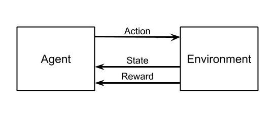
Reinforcement learning is about an agent learning to make a good sequence of decisions. The agent learns to make good decisions by exploring an environment and receiving feedback from the environment about the quality of each action. At each step, an agent must make a decision to move in a way that increases the expected reward. This sequential decision making is modeled as a Markov Decision Process (MDP) $\mathcal{M}:=(\mathcal{S}, \mathcal{A}, \mathcal{T}, \mathcal{R}, \gamma)$, where $\mathcal{S}$ represents a finite set of states, $\mathcal{A}$ represents a finite set of actions used to interact with the environment, $\mathcal{T}:\mathcal{S} \times \mathcal{A} \times \mathcal{S} \rightarrow[ 0, 1 ]$ is a stochastic transition function, where $T_{s, a}^{s^{\prime}}$ describes the probability of arriving in state $s^{\prime}$ after performing action $a$ in state $s$, $\mathcal{R} : \mathcal{S} \times \mathcal{A} \times \mathcal{S} \rightarrow \mathbb{R}$ is a scalar reward function, where $R_{s, a}^{s^{\prime}}$ denotes the expected reward after a state transition, and $\gamma$ is the discount factor controlling future versus immediate rewards. The future discounted reward of an agent at time $\hat{t}$ can be written as $R_{\hat{t}}=\sum_{t=\hat{t}}^{T} \gamma^{t-\hat{t}} r_{t}$, with $T$ marking the end of a learning episode and $r_{t}$ defining the immediate reward the agent receives at time $t$.

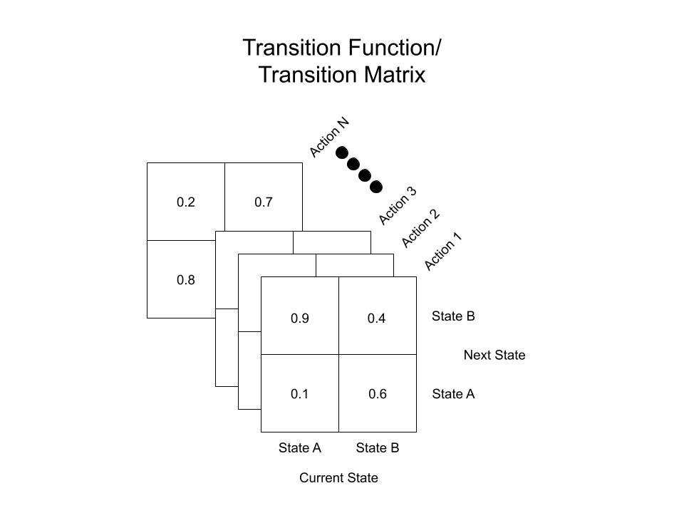
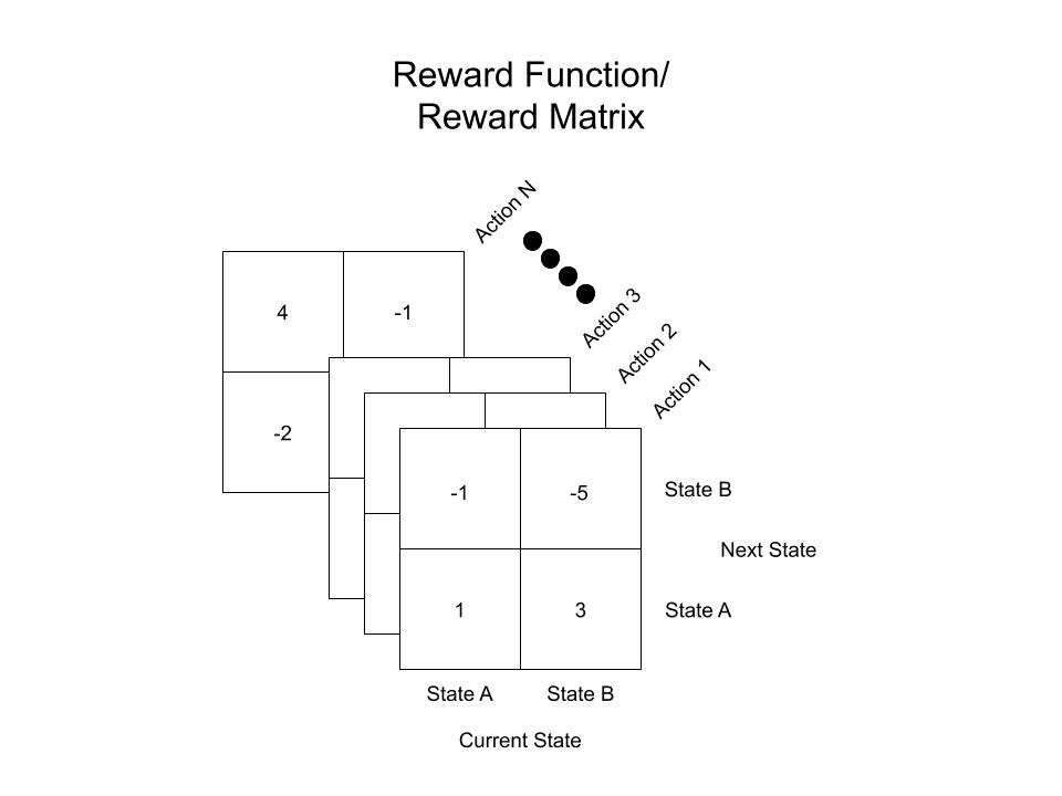
For example, the transition function $\mathcal{T}$ and reward function $\mathcal{R}$ of a two state MDP with an $\mathbf{N}$ dimensional action space may look like the following:

Q-Learning and Deep Q-Learning

Both of these topics deserve their own post/series of posts, but here I will only give a brief explanation of them to give context to the DQN network we designed. In Q-Learning, we learn want to learn the optimal action-value function, $Q^{*}(s, a)$, which denotes the ‘quality’ of an action in a given state. The $Q$ function can then be used to select an optimal action at every state:

$$ a = \arg\underset{a \in \mathcal{A}}{\max}{Q^{*}(s,a)} $$

In this work we utilize Deep Q-Learning which uses a deep neural network to approximate the action-value function: $Q(s,a) \approx Q(s,a;\theta)$. This network’s input is the current state of the agent, and the output is the $Q$ values for each action in the agent’s action space.

Framing Landmark Detection as an RL Problem

In order to do RL for landmark detection we need to answer three key questions: i) What is the reward function? ii) What is the state/observation space of the agent? and iii) What actions can the agent take in the environment?

Reward function: The reward is the difference in the euclidean distance of the agent to the landmark between the previous step and the current step. This can be written as: $r_{t} = d(p_{t-1}, x) - d(p_{t}, x)$, where $p_t$ is the agents position in $\mathbb{R}^n$ at time $t$, $x$ is the location of the target landmark in $\mathbb{R}^n$, and $d$ is the Euclidean distance function.

States: The state for our agent is the 29x29x29 cube of voxels (volumetric pixels) around the agent.

Action Space: The agent’s action space consists of moving left/right $(\pm x)$, anterior/posterior $(\pm y)$, and superior/inferior $(\pm z)$ by one voxel in the image. This allows the agent to easily traverse the entire 3D volume.

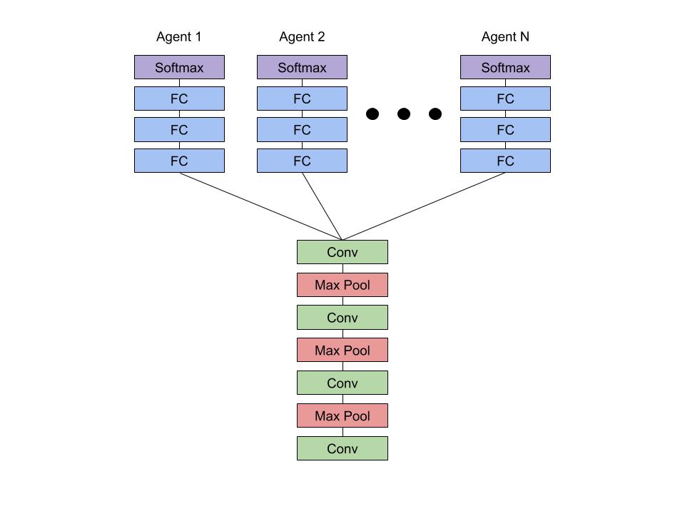
Sharing Representations w/ Hard Parameter Sharing

To detect multiple landmarks simultaneously, we need multiple agents to navigate their way through the image independently. Agents can work together in this process by sharing the weights of the convolutional layers. This technique of weight sharing, known as hard parameter sharing, leverages the similarity of all of the tasks to learn a common representation more rapidly.

Results

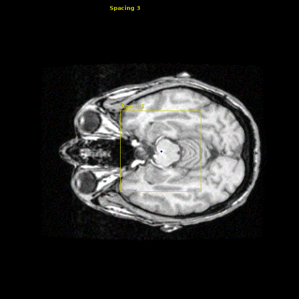
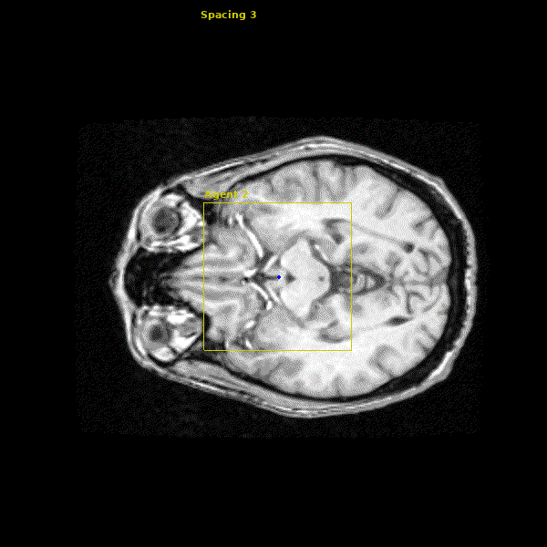
The network we made is able to accurately learn the trajectory and appearance of the landmarks of interest. We found that the network achieved accuracy on the order of 1-2mm. Below you can see three agents simulatenously detecting the Anterior Commissure (left), Left Eye (center), and Right Eye (right).